Mathematical optimization cheatsheet
In this cheatsheet, I will discuss many concepts that are essential in the analysis of optimization algorithms.
In the first part, I will recite the definitions of convexity, smoothness, and strong convexity, which are fundamental properties in the realm of convex optimization on differentiable functions. In the second part, we will relax to the case of non-differentiable functions and discuss subgradients, proximal operators and other concepts that are essential in the analysis of non-smooth optimization algorithms.
1. Convex optimization
Let us define a function $f: \text{dom}(f)\rightarrow \mathbb{R}$ with $\text{dom}(f) \subseteq \mathbb{R}^d$. We assume that $f$ is differentiable, meaning that the gradient $\nabla f(x) \in \mathbb{R}^d$ exists $\forall x \in \text{dom}(f)$.

1.1 Convexity
(a) Definition. A function $f$ is convex if its domain is a convex set and if for all $x, y \in \text{dom}(f)$ and $\theta \in [0, 1]$, we have
\[f(\theta x + (1-\theta)y) \leq \theta f(x) + (1-\theta)f(y)\]This definition is also known as the Jensen’s inequality. Oftentimes, it is more convenient to work with one of the following equivalent definitions:
(b) (First-order characterization) \(f(y) \geq f(x) + \langle \nabla f(x), y-x \rangle\)
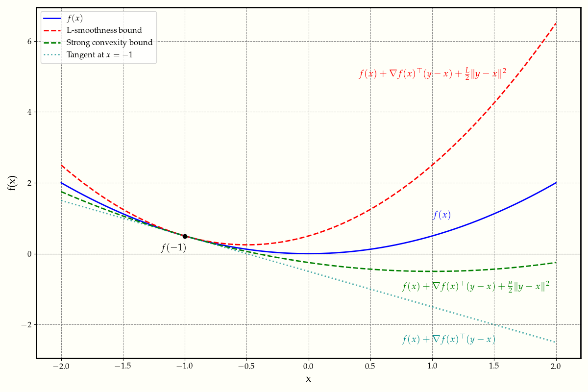
Geometrically, this definition implies that the function lies above its tangent line at any point (see Figure 1). Or, equivalently, the vector \((\nabla f(x), -1) \in \mathbb{R}^{d+1}\) defines a supporting hyperplane to the epigraph of \(f\) at \((x, f(x))\).
(c) (Second-order characterization) Suppose that $f$ is twice differentiable. A function $f$ is convex if its domain is a convex set and if for all $x \in \text{dom}(f)$, we have
\[\nabla^2 f(x) \succeq 0\]where $\nabla^2 f(x)$ is the Hessian matrix of $f$ at $x$.
(d) (Monotonicity of the gradient) A function $f$ is convex if its domain is a convex set and if for all $x, y \in \text{dom}(f)$, we have
\[\langle \nabla f(y) - \nabla f(x), y-x \rangle \geq 0\]1.2 Smooth functions
(a) Definition. Let $X\subseteq \text{dom}(f)$ be a convex set and let $L > 0$. A function $f$ is $L$-smooth on $X$ if for all $x, y \in X$, we have
\[f(y) \leq f(x) + \langle \nabla f(x), y-x \rangle + \frac{L}{2}\|y-x\|^2\]One can think of this definition as Lipschitz continuity of the gradient map. When $f$ is twice differentiable, smoothness implies that the largest eigenvalue of the Hessian is bounded by $L$, e.g. \(\|\nabla^2 f(x)\| \leq L\). If $f$ is $L$-smooth, then $f$ is also $L’$-smooth for all $L’ \geq L$. Alternatively, we can use the following equivalent definition:
(b) (Lipschitz continuity of the gradient) \(\| \nabla f(x) - \nabla f(y)\| \leq L\| x-y\|\) for all \(x, y \in X\).
(c) \(g(x) = \frac{L}{2} x^\top x - f(x)\) is convex.
(d) \(\langle \nabla f(x) - \nabla f(y), x-y \rangle \leq L\|x-y\|^2\) for all \(x, y \in X\).
These definitions are not actually equivalent, but they are related. We have the following relations:
\[[b] \Rightarrow [a] \Leftrightarrow [c] \Leftrightarrow [d]\]If $f$ is additionally convex, then \([a] \Rightarrow [b]\).
1.3 Strong convexity
(a) Definition. Let $X\subseteq \text{dom}(f)$ be a convex set and let $\mu > 0$. A function $f$ is $\mu$-strongly convex on $X$ if for all $x, y \in X$, we have
\[f(y) \geq f(x) + \langle \nabla f(x), y-x \rangle + \frac{\mu}{2}\|y-x\|^2\]The notion of strong convexity complements the notion of smoothness. Strong convexity implies that the function grows at least quadratically. Moreover, $f$ is strongly convex implies that $f$ is strictly convex and has a unique minimizer. And similarly to smoothness, if $f$ is $\mu$-strongly convex, then $f$ is also $\mu’$-strongly convex for all $\mu’ \leq \mu$. Alternatively, we can use the following equivalent definition:
(b) \(\| \nabla f(x) - \nabla f(y)\| \geq \mu\| x-y\|\) for all \(x, y \in X\).
(c) \(g(x) = f(x) - \frac{\mu}{2} x^\top x\) is convex.
(d) \(\langle \nabla f(x) - \nabla f(y), x-y \rangle \geq \mu\|x-y\|^2\) for all \(x, y \in X\).
The relations are as follows:
\[[b] \Leftarrow [a] \Leftrightarrow [c] \Leftrightarrow [d]\]Figure 1 above illustrates the complementary roles of smoothness and strong convexity in bounding the function values.
2. Non-smooth optimization
In this section, we define the function \(f\) similar to before, but we make no assumption of differentiability.
2.1 Non-smooth functions
(a) Definition. If \(f\) is not differentiable, or if the gradients of \(f\) exists but are not Lipschitz continuous, then we say that \(f\) is non-smooth. This definition is exactly the negation of the smoothness property. Examples of non-smooth functions include the absolute value function \(f(x) = |x|\), the hinge loss function \(f(x) = \max(0, 1-x)\), or many activation functions in neural networks such as the ReLU function \(f(x) = \max(0, x)\).
(b) Subgradients. A vector \(g \in \mathbb{R}^d\) is a subgradient of \(f\) at \(x\) if for all \(y \in \text{dom}(f)\), we have
\[f(y) \geq f(x) + \langle g, y-x \rangle\]We define a subdifferential \(\partial f(x)\) denoting the set of all subgradients of \(f\) at \(x\). Geometrically, \(g\) is a subgradient of \(f\) at \(x\) if the hyperplane defined by \((g, -1)\in\mathbb{R}^{d+1}\) supports the epigraph of \(f\) at \((x, f(x))\).
(c) Properties of subgradients.
- If \(f\) is differentiable at \(x\in \text{dom}(f)\), then \(\partial f(x) \subseteq \{\nabla f(x)\}\), meaning that the subdifferential either contains the gradient or is empty.
- If \(f\) is convex, then \(\partial f(x)\) is non-empty for all \(x\in \text{int(dom)}(f)\).
- If \(\text{dom}(f)\) is convex and \(\partial f(x) \neq \emptyset\) for all \(x\in \text{dom}(f)\), then \(f\) is convex.
- (Subgradient optimality condition) If \(\mathbf{0} \in \partial f(x)\), then \(x\) is a global minimum of \(f\).
2.2 Dual norms
(a) Definition. Given a general norm \(\|\cdot\|\), the dual norm \(\|\cdot\|_*\) is defined as
\[\|z\|_* = \max_{\|x\|\leq 1} \langle z, x \rangle\](b) Examples. In general, \(\|\cdot\|_p\) is the dual norm of \(\|\cdot\|_q\) if \(\frac{1}{p} + \frac{1}{q} = 1\).
- The dual norm of the \(\ell_1\) norm is the \(\ell_\infty\) norm.
- The dual norm of the \(\ell_2\) norm is the \(\ell_2\) norm.
(c) Interpretation of dual norms. (WIP)